
Even with the right indexes in place, spatial queries in SQL Server are often too slow – but they needn’t be.
Two of the most commonly found patterns of query in the spatial world are when you’re looking for the nearest thing to where you are (which I’ve written about before), and when you’re looking for the points that are within a particular boundary. This latter example is where I want to spend most of my time in this post.
A spatial index splits the world (for geography, or area for geometry) into a series of grids. The index essentially stores whether each point is inside each grid section or not, or for more complex types, whether it completely covers the grid section, whether it’s not in the grid section at all, or whether it’s partially in it. If we know that a particular grid section is completely covered by a polygon / multipolygon (I’m going to refer to polygons from here on, but it all applies to multipolygons too), then every point that is within that grid section must also be in that polygon. The inverse applies to a grid section which doesn’t overlap with a polygon at all – none of the points in that grid can be in that polygon.
More work is required if the overlap of the polygon and grid section is only partial.
Let’s assume we’ve got to the finest level of the grid system, and the polygon that we’re considering is partially overlapping the grid section. Now, we need to do some calculations to see if each point is within the polygon (or at least, the intersection of the grid section and the polygon). These calculations involve examining all the sections of the polygon’s boundary to see if each point is inside or outside.
Imagine trying to see if a particular point is within the coastline of Australia or not, and just rely on our eyes to be able to judge whether an answer is ‘easy’ or ‘hard’.

If we’re zoomed out this much, we can easily tell that a point near the border of South Australia and Northern Territory (near where it says ‘Australia’ in red) is within the coastline, or that a point half way between Tasmania and Victoria is not. To know whether some arbitrary point near Adelaide is within the coastline or not – I can’t tell right now. I’m going to need to zoom in more.

Now, if my point of interest is near Murray Bridge, or in the sea between Kangaroo Island and the mainland, then I can tell my answer. But somewhere slightly northwest of Adelaide, and again, we need to zoom. But notice here that we can see a lot more detail about the coastline than we could see before. Parts of the coastline that seemed like relatively simple now show a complexity we hadn’t started to consider.
If we zoom again, we see that the coastline to the northwest of Adelaide is frustratingly complex.

And this doesn’t stop as we keep zooming.


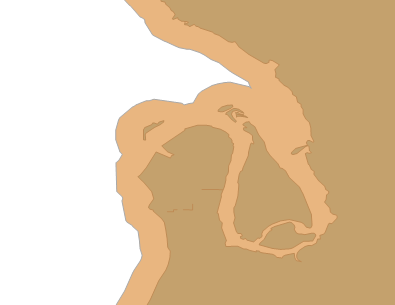
The area around the Port River here is full of man-made structures, which can be defined relatively easily at some zoom level. A natural coastline is trickier (go back a few images to see the zoomed out version of this next one).

Here we see a complexity that could just keep going. Each of these bays would have their own level of complexity, and as we zoom, we would see that the complexity just keeps going. The crinkliness of coastlines becomes like a fractal, that can keep zooming further and further, like in the animated GIF here (which is on a loop, but I think demonstrates the point well enough). It’s supposedly an illusion, but it’s really a basic property of fractals.
 (Image from http://www.moillusions.com/infinite-zoom-coast-illusion/)
Benoit B. Mandelbrot’s work in fractals shows a pattern which is probably a more familiar ‘infinite zoom’ concept.
 (Image from http://commons.wikimedia.org/wiki/File:Mandelbrot_color_zoom.gif)
Coastlines don’t actually let us zoom in infinitely, because we can’t go far part the detail in atoms, but we do need to consider how much detail we choose to define in our polygons.
If I consider a dataset I have of South Australian spatial data, and I query the UnionAggregate of the different postcode areas, I get a geography value of the whole state.

There are over 26,000 points defining this area (I didn’t count them, I used the STNumPoints method). If I convert it into a string (using .ToString()), I get a result which is over a million characters long. This is going to take a lot of effort to use in real queries.
But how much detail do I actually need?
One of the spatial methods is called Reduce(). It simplifies the shapes involved.
If I use Reduce(50), then it reduces the number of points by about half. But at the zoom level we can see at this point, we might not care at all.

If I Reduce(250), the number of points comes down to about 4000.

This isn’t necessarily good though. Reducing even further can start to distort the borders so much that we end up making mistakes. A point that is within the Reduced polygon might not be in our original one, and vice versa.
At Reduce(10000) I have under 400 points.

At Reduce(50000) you can clearly see changes. Kangaroo Island has been simplified too much. The peninsulas have become remarkably triangular, and we would be making mistakes.

Mistakes will come as soon as we Reduce the number of points at all. Despite the fact that at the level shown above, we could see no discernible different between the original set and Reduce(50), if we zoom in we can see that even Reduce(50) is a problem.

You can clearly see that the crinkliness has been reduced, but that this could make the results of any query change. It would perform better, but it would be wrong.
However – it would only be wrong near the borders. We can use this…
Let me tell you about three other methods – STBuffer(@d), BufferWithCurves(@d), BufferWithTolerance(@d, @t, @r). These put a buffer around our polygon. If we have buffered enough, and then we Reduce, we can make sure that we get no false negatives from our check. So that anything that outside this area is definitely outside the original.
BufferWithCurves produces a buffer shape using curves rather than points, which can offer some nice optimisations, but buffering coastlines using BufferWithCurves is very memory-intensive, and you may even find you are unable to produce this buffer.
BufferWithTolerance is like having a Reduce built into the buffer – which sounds ideal, but I found that even with a very high tolerance I was still getting too many points for my liking. With a buffer of 1000, and tolerance of 250, I still had nearly 20,000 points. The things that look like curves in the image below are actually made up of many points.
So I’m choosing a Reduced STBuffer instead.
With a large enough value for STBuffer, and sufficiently small value for Reduce, I can make a simple border, and can use STDifference to confirm that it completely surrounds my original polygon. With not much effort, I can find some values that work enough. Notice that there are only seven points in the image below, whereas the BufferWithOverflow version has hundreds.
select @SApolygon union all select @SApolygon.STBuffer(500).Reduce(500)

The query below confirms that no part of the original land is outside my buffered and reduced area, showing zero points in the STDifference, and is what I used to find appropriate values for buffering and reducing.
select @SApolygon.STDifference(@SApolygon.STBuffer(@reducefactor).Reduce(@reducefactor)).STNumPoints();

Having defined an area that can have no false negatives, we can flip it around to eliminate false positives. We do this by buffering and reducing the inverse (which we find using ReorientObject()). I actually found that buffering by 1000 was needed to make sure there was no overlap (the second query below confirms it – the first query is just to overlay the two images).
select @SApolygon union all select @SApolygon.ReorientObject().STBuffer(1000).Reduce(500).ReorientObject();
select @SApolygon.ReorientObject().STBuffer(1000).Reduce(500).ReorientObject().STDifference(@SApolygon).STNumPoints(); –must be be zero

With a zero for the second query above, we have defined an area for which there are no false positives.
Now I know that points within the ‘no false positives’ area are definitely within my original polygon, and that points within the ‘no false negatives’ area are definitely not. The area between the two is of more interest, and needs checking against the complex coastline.

Now let’s play with some better queries to show how to do this.
Let’s create a table of areas. I’m going to use computed columns (which must be persisted to be useful) for the ‘no false negatives’ and ‘no false positives’ areas, although I could’ve done this manually if I wanted to experiment with buffers and tolerances on a per-area basis. Let’s also create a table of points, which we’ll index (although I’ll also let you know how long the queries took without the index).
|
1 2 3 4 5 6 7 8 9 10 11 12 13 |
create table dbo.areas (id int not null identity(1,1) primary key, area geography, nofalseneg as area.STBuffer(500).Reduce(500) persisted, nofalsepos as area.ReorientObject().STBuffer(1000).Reduce(500).ReorientObject() persisted ); go create table dbo.points (id int not null identity(1,1) primary key, point geography ); go create spatial index ixSpatialPoints on dbo.points(point); |
And we’ll put some data in. Our SA outline in the areas, and the points from AdventureWorks2012’s list of addresses – 19614 points.
|
1 2 3 4 5 6 7 |
insert dbo.areas (area) select geography::UnionAggregate(geom) from postcodes.dbo.postcodes go insert dbo.points (point) select SpatialLocation from AdventureWorks2012.person.Address; |
Putting the data in took some time. The 19,614 points took over about 5 seconds to get inserted, but the 1 area took 25 seconds. STBuffer() takes a while, and this is why having these computed columns as persisted can help so much.
The query that we want to solve is:
|
1 2 3 |
select p.* from areas a join points p on p.point.STIntersects(a.area) = 1; |
This returns 46 rows, and it takes 4 seconds (or 3.5 minutes without the index).
…whereas this query takes less than a second (or 20 seconds without the index):
|
1 2 3 |
select p.* from areas a This query Intersects(a.nofalsepos) = 1; |
But it only returns 44 rows, because we’re only including the points that are in the “no false positives” area.
This query returns 47 rows. We’re counting the points that are in the “no false negatives” area, which is a larger area than we want.
|
1 2 3 |
select p.* from areas a join points p on p.point.STIntersects(a.nofalseneg) = 1; |
It also runs in under a second (or 20 seconds without the index).
By now hopefully you see where I’m getting at…
What I need is the list of points that are inside ‘nofalsepos’, plus the ones that inside ‘nofalseneg’, but not inside ‘nofalsepos’, that have also been checked against the proper area.
|
1 2 3 4 5 6 7 8 9 10 |
select p.* from areas a join points p on p.point.STIntersects(a.nofalsepos) = 1 union all select p.* from areas a join points p on not p.point.STIntersects(a.nofalsepos) = 1 and p.point.STIntersects(a.nofalseneg) = 1 and p.point.STIntersects(a.area) = 1; |
This query takes approximately 1 second (or 40 without the index).
But it’s complex – and that’s unfortunate, but we can figure this out using a view.
|
1 2 3 4 5 6 7 8 9 10 11 |
create view dbo.PointAreaOverlap as select p.id as pointid, p.point, a.id as areaid, a.area from areas a join points p on p.point.STIntersects(a.nofalsepos) = 1 union all select p.id as pointid, p.point, a.id as areaid, a.area from areas a join points p on not p.point.STIntersects(a.nofalsepos) = 1 and p.point.STIntersects(a.nofalseneg) = 1 and p.point.STIntersects(a.area) = 1; |
, which we can query using much simpler code such as:
|
1 2 3 |
select pointid, point from dbo.PointAreaOverlap where areaid = 1; |
Coastlines, or any complex spatial values, can make for poor performance, even with indexes in place. To improve performance, you could consider Reduce() to have it run quicker, although you’ll need to take some additional steps to guarantee correctness.
And in case you were wondering what the “B.” in “Benoit B. Mandelbrot” stands for… it stands for “Benoit B. Mandelbrot”.


This Post Has One Comment
There’s another way..
Tesselate the polygon yourself. The relationship between how quickly the spatial query works (across all the rdbms’) is how much extra work the 2nd pass (after .Filter) has to do to get rid of the false positives.
By slicing your complex polygon into simpler, more rectangular shapes you remove the false positive ‘white space’ around your complex polygon. There’s some of my code and more info here – https://social.msdn.microsoft.com/Forums/sqlserver/en-US/78132bca-2a95-45c1-b93c-64c83827dc4f/sql-2k8r2-any-performance-hints-for-bulk-loading-data-from-spatialgis-db-into-a-data-warehouse?forum=sqlspatial
I’d be curious to see how the TVFs compare to the approaches you outlined above. Mine doesn’t scale too well; the overhead of the TVF recursively sliciing the polygons becomes obscene once you start throwing a dozen or so complex polygons at it.
I have a .netclr version of it as well that’ll eventually make it online. All coded and working, just the doco left… This one does scale very well